Physical Address
Lahore, Punjab, Pakistan
Physical Address
Lahore, Punjab, Pakistan

From fundamentals to fieldbus — a complete reference for practicing engineers, fresh graduates, and interview preparation. Covers IEC standards, industrial protocols, and real-world applications.
Instrumentation engineering is a branch of engineering that deals with the design, installation, calibration, and maintenance of instruments and control systems used to measure and control physical variables such as pressure, temperature, level, flow, and composition in industrial processes.
It forms the sensory and control backbone of industries like oil & gas, power generation, pharmaceuticals, water treatment, and manufacturing. An instrumentation engineer ensures that process variables are measured accurately and that control systems respond correctly to maintain safe and efficient operations.
| Sensor | Transducer |
|---|---|
| Detects or senses a physical quantity (temperature, pressure, level, etc.) | Converts one form of energy or physical quantity into another, usually an electrical signal |
| May produce a non-electrical or electrical response | Produces an output proportional to the measured quantity (electrical or mechanical) |
| Example: RTD, Thermistor, LDR, Bourdon Tube | Example: Transmitter, LVDT, Piezoelectric Sensor |
| A sensor is the sensing element of a measurement system. | A transducer consists of a sensing element and an energy-conversion mechanism. |
A transmitter is a device that converts the output of a sensor into a standardized signal (typically 4–20 mA DC or digital HART) suitable for transmission over long distances to a control system (DCS/PLC).
A pressure transmitter, for example, contains a sensing element (capacitive cell or piezoelectric) plus electronics that output a 4–20 mA signal proportional to the measured pressure range.
The 4–20 mA current loop is an industrial standard where 4 mA represents 0% of process range and 20 mA represents 100%. It is a current signal, not voltage, which gives it several advantages:
| Term | Definition | Example |
|---|---|---|
| Accuracy | Closeness of measurement to the true/reference value | Reading 100.2 bar when true value is 100 bar → 0.2% accurate |
| Precision | Consistency of repeated measurements (regardless of whether they're correct) | Always reading 98 bar consistently — precise but not accurate |
| Repeatability | Same result when same input applied multiple times under same conditions | Five consecutive readings all give 99.8 bar |
Hysteresis is the difference in output readings of an instrument when the same input value is approached from increasing versus decreasing direction. It is caused by mechanical friction, backlash in gears, magnetic effects, or elastic deformation in sensing elements.
For example, if a pressure gauge reads 50.5 bar when pressure is rising to 50 bar, but reads 49.6 bar when falling back to 50 bar — the hysteresis is 0.9 bar.
Zero calibration adjusts the instrument output at the lowest end of its range (0% → 4 mA). If the instrument reads 4.3 mA at zero input, the zero is adjusted down.
Span calibration adjusts the instrument output at the highest end of its range (100% → 20 mA). If the instrument reads 19.5 mA at full input, the span is adjusted up.
The procedure is typically: apply zero input → adjust zero → apply full-scale input → adjust span → repeat until both are within tolerance.
A P&ID (Piping & Instrumentation Diagram) is an engineering drawing that shows all process equipment, piping, instrumentation, control loops, and interlocks in a process plant. It is the master reference document for instrument engineers.
Key symbol categories (per ISA 5.1):
First letter = measured variable (F=Flow, P=Pressure, T=Temperature, L=Level). Subsequent letters = function (T=Transmitter, C=Controller, V=Control Valve, S=Switch, I=Indicator).
| Analog Signal | Digital Signal |
|---|---|
| Continuous variation (e.g., 4–20 mA, 0–10V) | Discrete states only (ON/OFF, 0 or 1) |
| Susceptible to noise and signal degradation | Highly immune to noise |
| Simple wiring, easy to understand | Can carry diagnostic data (HART, FF, Profibus) |
| Examples: 4–20 mA, 1–5V, 0–10V | Examples: HART, Modbus, Foundation Fieldbus |
| One variable per wire pair | Multiple variables on one cable (fieldbus) |
Signal conditioning is the process of manipulating an analog or digital signal to prepare it for further processing or transmission. It bridges the gap between raw sensor output and the input requirements of a control system.
Common signal conditioning functions:
A control loop is a system that measures a process variable and adjusts a manipulated variable to achieve and maintain a desired setpoint.
| Open Loop | Closed Loop |
|---|---|
| No feedback from process output | Continuous feedback from process output |
| Controller doesn't know if setpoint is reached | Controller corrects based on error (SP – PV) |
| Simple, inexpensive | More complex but accurate and self-correcting |
| Example: timer-controlled pump | Example: flow controller with PID |
In closed-loop: Sensor → Transmitter → Controller (PID) → Final Control Element (valve) → Process → back to Sensor
Rangeability (also called turndown ratio) is the ratio of the maximum measurable value to the minimum measurable value of an instrument while still maintaining acceptable accuracy.
A higher rangeability means the instrument can accurately measure over a wider range of process conditions, which reduces the need for multiple instruments on varying flows.
Turndown ratio is the ratio of the maximum flow (or measurement) to the minimum flow at which the instrument maintains its specified accuracy. It is the same concept as rangeability.
| Meter Type | Typical Turndown |
|---|---|
| Orifice Plate | 3:1 to 5:1 |
| Vortex Flowmeter | 10:1 to 20:1 |
| Coriolis Flowmeter | 100:1 or more |
| Electromagnetic Flowmeter | 40:1 or more |
| Intrinsic Safety (Ex i) | Explosion-Proof (Ex d) |
|---|---|
| Limits energy in circuit to below ignition level | Contains explosion within the enclosure |
| Prevents ignition from occurring | Prevents ignition from escaping |
| Requires barriers/isolators in safe area | Heavy, robust enclosure with flame-path joints |
| Suitable for Zones 0, 1, 2 (with ia, ib certification) | Suitable for Zone 1 and Zone 2 |
| Low power devices only (transmitters, sensors) | Can be used for higher power equipment (motors) |
| Can be worked on live in hazardous area | Must be de-energized before opening |
| Type | Reference | Example |
|---|---|---|
| Absolute Pressure | Perfect vacuum (0 bar abs) | Atmospheric = 1.013 bar abs |
| Gauge Pressure | Local atmospheric pressure | Tyre = 2 bar g (above atmosphere) |
| Differential Pressure | Another process point | DP across orifice plate = 250 mbar |
| Vacuum Pressure | Below atmospheric | Condenser vacuum = −0.3 bar g |
A Bourdon tube is a curved, hollow, oval cross-section metal tube sealed at one end. When pressure is applied at the open end, the tube tends to straighten out. This mechanical deflection is transmitted through a gear-and-link mechanism to a pointer on a calibrated dial.
Operating range: typically 0.6 bar to 1,000 bar. Accuracy: typically ±1% to ±0.5% FS.
A DP transmitter measures the difference in pressure between two points (High side and Low side) and outputs a 4–20 mA signal proportional to this difference.
Applications:
Key selection parameters:
| Pressure Switch | Pressure Transmitter |
|---|---|
| Provides ON/OFF discrete output | Provides continuous 4–20 mA analog output |
| Activates at a set trip point | Measures across full range continuously |
| Used for alarms and shutdowns (ESD) | Used for monitoring and control |
| Lower cost, simple wiring | Higher cost, more information |
| No feedback on process between trips | Full process visibility at all times |
A diaphragm seal (also called a chemical seal or remote seal) is a device with a flexible diaphragm that isolates the pressure transmitter from direct contact with the process fluid. The system is filled with a fill fluid (typically silicone oil, glycerin, or capillary oil) that transmits pressure from the diaphragm to the transmitter.
Used when:
Static pressure error (also called line pressure effect) is the change in DP transmitter zero or span output caused by the absolute static pressure applied equally to both the High and Low process connections.
Even though DP = 0 (equal pressure on both sides), the high line pressure can slightly deform the sensing capsule, causing a false output. This is specified by manufacturers as:
This error is significant in high-pressure flow metering applications and must be compensated or accounted for in the accuracy budget.
Equipment needed: Calibrated pressure source (hand pump or deadweight tester), HART communicator or digital multimeter, reference standard.
Procedure:
Over-range protection is the ability of a pressure instrument to withstand pressure levels exceeding its calibrated range without damage or loss of calibration. It is specified as a multiple of the Upper Range Limit (URL).
For example, a transmitter with URL of 10 bar and 2× overpressure protection can withstand 20 bar without damage. Modern smart transmitters typically have overpressure ratings of 2× to 10× the URL.
| Method | Principle | Typical Use |
|---|---|---|
| DP Transmitter | Hydrostatic pressure (ρgh) | Open/closed tanks, liquids |
| Float | Buoyancy | Simple tank indication, switches |
| Displacer | Buoyancy force change | Interface level, high pressure/temp |
| Radar (Non-contact) | Microwave time-of-flight | Liquids and solids, agitated surfaces |
| Guided Wave Radar | Microwave along probe | Interface, foam, low dielectric fluids |
| Ultrasonic | Sound wave echo | Open tanks, non-contact, solids |
| Capacitance | Dielectric change | Liquids, solids, slurries |
| Nuclear (Radiometric) | Gamma ray attenuation | Extreme conditions, external mounting |
A DP level transmitter measures the hydrostatic pressure created by the liquid column above the low pressure tap. As liquid level rises, the pressure on the HP side increases, and the DP signal increases proportionally.
For an open tank: HP tap at bottom, LP tap vented to atmosphere. For a closed/pressurized tank: HP at bottom, LP connected to vapor space at top (wet or dry leg configuration required).
Used for closed/pressurized tanks where the LP side must be connected to the vapor space:
Radar level transmitters emit microwave signals (typically 6 GHz, 26 GHz, or 79 GHz) that reflect off the liquid surface. The time taken for the echo to return is converted to distance and then level.
| FMCW (Frequency Modulated Continuous Wave) | Pulse Radar |
|---|---|
| Continuously varies frequency | Emits short microwave pulses |
| Measures frequency difference between sent and received | Measures time-of-flight of pulse |
| Higher accuracy (±1–2 mm) | Lower accuracy (±3–5 mm) |
| Better for short distances and agitated surfaces | Suitable for longer range |
| Higher cost | Lower cost |
| Guided Wave Radar (GWR) | Non-Contact Radar |
|---|---|
| Probe inserted into tank guides signal along its length | Antenna emits free-space microwave beam |
| Works with low dielectric constant fluids (hydrocarbons) | Needs adequate dielectric constant (εr > 1.5 min) |
| Not affected by vapor, foam, or condensation | Foam or heavy vapor can attenuate signal |
| Can measure interface between two liquids | Measures only top surface of liquid |
| Probe length limits tank height | Can measure up to 30–40 m range |
| Risk of probe damage in agitated/slurry media | No moving parts, no contact with media |
A displacer-type level transmitter operates on the principle of Archimedes — buoyancy. A heavy cylindrical displacer is submerged in the liquid. As liquid level rises, the buoyancy force on the displacer increases, reducing the apparent weight. This change in force (via a torque tube or spring) is converted to a 4–20 mA output signal.
Advantage: Excellent for interface level measurement, high-pressure/high-temperature applications, and fluids with varying density. Disadvantage: Requires calibration with actual process fluid density.
A float switch is a simple level detecting device consisting of a hollow float (usually polypropylene, SS, or PVC) attached to a stem or cable. As the liquid level rises or falls, the float rises or falls, actuating a magnetic reed switch or mechanical switch at a predetermined level.
It provides a discrete ON/OFF output used for high level alarm (HLA), low level alarm (LLA), or pump start/stop control. Simple, reliable, low-cost but provides only a single point measurement and has moving parts that can stick or corrode.
| Use Ultrasonic When… | Use Radar When… |
|---|---|
| Open tanks with no heavy vapors | Heavy vapors, steam, or condensing atmosphere |
| Water, sewage, or non-volatile liquids | Hydrocarbons, solvents, pressurized vessels |
| Lower cost is a priority | Accuracy is critical (±1–2 mm) |
| Solids (silos) — short range | Tall tanks, boiling surfaces, agitation present |
| Temperature is near ambient | High temperature applications |
Interface level measurement is the detection of the boundary (interface) between two immiscible liquids with different densities within the same vessel. Common applications include oil-water separators, API separators, desalters, and solvent extraction vessels.
Technologies used:
| Type | Examples | Principle |
|---|---|---|
| Differential Pressure | Orifice plate, Venturi, Flow nozzle | Pressure drop across restriction |
| Velocity-based | Electromagnetic, Vortex, Turbine, Ultrasonic | Velocity × Area = Volumetric flow |
| Mass Flow | Coriolis, Thermal mass | Direct mass measurement |
| Positive Displacement | Oval gear, Nutating disk | Fixed volume per rotation |
| Open Channel | Weir, Flume (Parshall) | Head-flow relationship |
An orifice plate is a flat plate with a precisely machined hole (orifice) inserted in a pipe. As fluid passes through the restriction, velocity increases and pressure drops (Bernoulli's principle). A DP transmitter measures this pressure difference, and flow is calculated from it.
Limitations:
Vena contracta is the point downstream of an orifice plate (or any flow restriction) where the jet of fluid reaches its minimum cross-sectional area and maximum velocity. At this point, the static pressure is at its minimum.
The vena contracta occurs slightly downstream of the physical orifice opening because the fluid continues to converge after passing through the orifice. The location of the vena contracta (typically 0.3D to 0.5D downstream) is important for pressure tap placement in orifice plate designs (vena contracta taps).
| Volumetric Flow | Mass Flow |
|---|---|
| Volume of fluid per unit time (m³/h, L/min) | Mass of fluid per unit time (kg/h, t/h) |
| Changes with temperature and pressure | Independent of temperature and pressure |
| Suitable for liquids at steady conditions | Essential for custody transfer and gas flow |
| Measured by: orifice, mag, vortex, turbine | Measured by: Coriolis, thermal mass |
A Coriolis meter uses two vibrating tubes through which the process fluid flows. When fluid is flowing, the Coriolis force (resulting from rotation + linear velocity) causes the tubes to twist. The degree of twist is directly proportional to the mass flow rate.
What it measures directly:
Accuracy: ±0.05% to ±0.1% of reading. Turndown: 100:1 or more. No straight pipe run required. Suitable for highly viscous fluids and non-Newtonian fluids.
A magnetic flowmeter (magmeter) works on Faraday's Law of electromagnetic induction. A magnetic field is applied across the pipe, and as conductive fluid flows through, an EMF (voltage) is induced proportional to the fluid velocity.
Requirements: Fluid must be electrically conductive (minimum 5–20 µS/cm conductivity)
Suitable fluids: Water, acids, bases, slurries, pulp, wastewater, food products
NOT suitable for: Hydrocarbons, gases, pure water (DI water), steam
Advantages: No pressure drop, no moving parts, bidirectional, suitable for slurries
A vortex flowmeter contains a bluff body (shedder bar) in the flow stream. Fluid passing the bluff body creates alternating vortices downstream (von Kármán vortex street). The frequency of these vortices is directly proportional to the fluid velocity.
Suitable for: steam, gases, clean liquids. Not suitable for: very low flow velocities (below Reynolds number ~10,000), viscous fluids, slurries, or pulsating flow. Turndown: typically 10:1 to 20:1.
A turbine flowmeter uses a multi-blade turbine rotor mounted axially in the flow stream. As fluid passes, it spins the rotor at a speed proportional to flow velocity. A magnetic pickup (or optical sensor) counts blade passes per unit time, generating pulses that correspond to volumetric flow rate.
Key features: High accuracy (±0.25%–0.5%), good for clean, low-viscosity liquids and gases, wide turndown (10:1). Not suitable for dirty, viscous, or abrasive fluids (bearing wear).
| Transit-Time (Time-of-Flight) | Doppler |
|---|---|
| Measures time difference of sound pulse traveling upstream vs downstream | Measures frequency shift of sound reflected by particles/bubbles |
| Requires clean fluid (no bubbles or particles) | Requires particles or bubbles (>100 ppm, >75 µm) |
| High accuracy (±0.5–1%) | Lower accuracy (±2–5%) |
| Suitable for water, clean hydrocarbons, gases | Suitable for slurries, dirty water, sewage |
| Can be clamp-on (non-invasive) | Usually clamp-on |
Beta ratio (β) is the ratio of the orifice bore diameter (d) to the internal pipe diameter (D).
Effect of beta ratio:
Key selection criteria:
| RTD (Resistance Temperature Detector) | Thermocouple |
|---|---|
| Resistance increases with temperature | Generates voltage (EMF) from junction of two metals |
| High accuracy (±0.1°C to ±0.3°C) | Lower accuracy (±1°C to ±2°C) |
| Better repeatability and stability | Less stable over time (drift) |
| Slower response time | Faster response time |
| Range: −200°C to +850°C (Pt100) | Range: −200°C to +1800°C (type B) |
| Requires excitation current (self-heating error) | Self-generating (no excitation needed) |
| More expensive | Less expensive, simpler |
| Suitable for lower temperatures, high accuracy needs | Suitable for high temperatures (>600°C) |
| Type | Metals | Range | Application |
|---|---|---|---|
| J | Iron / Constantan | −210 to +1200°C | General industrial, reducing atmosphere |
| K | Chromel / Alumel | −200 to +1372°C | Most common general-purpose type |
| T | Copper / Constantan | −270 to +400°C | Cryogenic, food industry |
| E | Chromel / Constantan | −270 to +1000°C | Highest EMF output, good for sub-zero |
| N | Nicrosil / Nisil | −270 to +1300°C | Replacement for K, better stability |
| R | Pt-13%Rh / Pt | 0 to +1768°C | High temperature, lab/furnaces |
| S | Pt-10%Rh / Pt | 0 to +1768°C | High temperature, ITS-90 reference |
| B | Pt-30%Rh / Pt-6%Rh | +600 to +1820°C | Highest temperature, glass furnaces |
A Pt100 is a platinum RTD (Resistance Temperature Detector) with a resistance of exactly 100 Ω at 0°C. It follows the Callendar-Van Dusen equation where resistance increases linearly with temperature (with a small non-linear correction).
Pt100 is the most widely used RTD in industry due to its excellent linearity, stability, repeatability, and wide availability of compatible transmitters and head-mount transmitters per IEC 60751.
A thermocouple generates an EMF proportional to the temperature difference between the hot junction (measuring end in process) and the cold junction (reference end at the instrument/transmitter).
The EMF tables (IEC 60584) are referenced to 0°C cold junction. If the actual cold junction is at 25°C (room temperature), the measured voltage corresponds to (hot − 25°C), not (hot − 0°C). This error must be compensated.
Cold Junction Compensation (CJC) measures the actual temperature at the cold junction (using an RTD or thermistor built into the transmitter/instrument) and electronically adds the correction to give the true hot junction temperature.
A thermowell is a closed-end tube installed permanently into a pipe or vessel that allows a temperature sensor to be inserted, removed, or replaced without shutting down or depressurizing the process.
Key purposes:
Types: Straight, stepped (tapered), tapered — selected based on wake frequency analysis (ASME PTC 19.3 TW) to avoid resonance with flow-induced vortex shedding.
Thermowell insertion length (U-length) should be sufficient to place the sensor tip at the center of the pipe (or at least 1/3 of the pipe diameter from the opposite wall) to measure the bulk fluid temperature.
Insertion length must also be checked against ASME PTC 19.3 TW for wake frequency calculation to ensure the thermowell natural frequency is above the vortex shedding frequency at maximum flow velocity.
| Configuration | How It Works | Accuracy | Use Case |
|---|---|---|---|
| 2-wire | Lead resistance added directly to measurement, no compensation | Lowest (error from cable resistance) | Short cable runs only, non-critical |
| 3-wire | Third wire allows partial lead resistance compensation (assumes equal lead resistance) | Medium (good for most industrial use) | Most common industrial standard |
| 4-wire | Two current leads, two voltage sense leads — fully eliminates lead resistance effect | Highest (laboratory/precision) | Custody transfer, high accuracy requirements |
An infrared (pyrometer) temperature sensor measures temperature without physical contact by detecting the infrared radiation emitted by all objects above absolute zero. The power of emitted radiation follows the Stefan-Boltzmann law.
Used when:
Key parameter — Emissivity (ε): Must be set correctly for the target material. Shiny metals have low emissivity (ε ≈ 0.1) while blackbody surfaces have ε ≈ 1. Wrong emissivity setting causes significant measurement error.
A control valve is a power-operated device that modulates the flow of a process fluid by varying the size of the flow passage. It is the final control element in a control loop, directly manipulating the process variable.
Main components:
| Parameter | Globe Valve | Butterfly Valve | Ball Valve |
|---|---|---|---|
| Control characteristics | Best (linear/eq.%) | Good (modified equal%) | Poor (quick-opening) |
| Pressure drop | High | Low | Low (full bore) |
| Rangeability | 50:1 | 20:1 | 10:1 |
| Size range | ½" to 24" | 2" to 120"+ | ½" to 24" |
| Cost | Higher | Lowest | Medium |
| Best for | Throttling, precise control | Large diameter, low pressure | On/off, moderate control |
Cv is the flow coefficient of a control valve, defined as the number of US gallons per minute of water at 60°F that will flow through the valve with a pressure drop of 1 psi across it at full open position.
Cv is used to size control valves. The required Cv is calculated at maximum, normal, and minimum flow conditions. The selected valve must have a Cv range that covers the entire operating range with adequate rangeability.
| Air-to-Open (ATO) / Fail-Close (FC) | Air-to-Close (ATC) / Fail-Open (FO) |
|---|---|
| Valve opens as air signal increases | Valve closes as air signal increases |
| On air/signal loss → valve CLOSES | On air/signal loss → valve OPENS |
| Safe fail position = CLOSED | Safe fail position = OPEN |
| Used where closing on failure is safe (fuel gas, flammables) | Used where opening on failure is safe (cooling water, vent to flare) |
The fail-safe position is the position a control valve defaults to when the instrument air supply or control signal is lost. It is chosen based on process safety analysis to minimize risk in the event of instrument failure.
Options: Fail Open (FO), Fail Close (FC), Fail in Last Position (FL/Lock)
Examples:
Valve rangeability is the ratio of the maximum controllable flow to the minimum controllable flow through the valve while still maintaining the specified inherent flow characteristic.
This is different from the installed rangeability, which is affected by the system resistance curve. High rangeability means the valve can control accurately over a wider range of process flows, reducing the need for multiple valves.
| Linear Trim | Equal Percentage Trim |
|---|---|
| Flow increases proportionally with valve travel (constant gain) | Equal increments of travel produce equal percentage changes in existing flow |
| Cv increases linearly with stem position | Cv increases exponentially with stem position |
| Best when valve pressure drop is constant (most of system ΔP) | Best when valve takes small % of total system ΔP (pumped systems) |
| Open channel, gravity flow systems | Most common in process industry (pumped, heat exchanger applications) |
Flashing: Occurs when the downstream pressure of the valve falls below the fluid's vapor pressure. A portion of the liquid permanently vaporizes — mixed liquid-vapor flow exits the valve. Results in reduced capacity and erosion.
Cavitation: Occurs when pressure drops below vapor pressure at the vena contracta (inside the valve) — bubbles form — then pressure recovers above vapor pressure downstream, causing bubbles to violently implode. This implosion causes severe pitting, noise, vibration, and material damage to the valve trim.
A valve positioner is a device that receives the control signal (4–20 mA from DCS/PLC) and accurately positions the valve stem by manipulating the instrument air supply to the actuator. It compares the commanded position to the actual stem position (via feedback linkage) and adjusts air output to eliminate any error.
Benefits of using a positioner:
| Pneumatic Positioner | Electro-Pneumatic Positioner |
|---|---|
| Input signal: 3–15 psi pneumatic | Input signal: 4–20 mA electrical |
| Purely mechanical/pneumatic internals | Contains I/P converter + positioner electronics |
| No electrical power needed | Requires 24V DC power for electronics |
| Simpler, more robust in harsh environments | Compatible with modern DCS/PLC 4–20 mA output |
| Rarely used in new designs | Standard in modern plants |
| PLC | DCS | SCADA |
|---|---|---|
| Programmable Logic Controller | Distributed Control System | Supervisory Control and Data Acquisition |
| Fast discrete & sequential control | Continuous process control, regulatory loops | Remote monitoring over large geographic areas |
| Single panel, one or few processors | Multiple controllers distributed across plant | Central software + remote field units (RTUs) |
| Packaging, conveyor, ESD, safety systems | Refineries, power plants, chemical plants | Pipelines, water networks, power grids |
| Ladder logic, FBD, ST programming | FBD, high-level config tools | HMI software (iFIX, WinCC, Ignition) |
| Scan time: <1 ms to 10 ms | Scan time: 100 ms to 500 ms typical | Communication latency seconds to minutes |
A PID controller is the most common feedback controller in process control. It calculates a control output based on three terms acting on the error (Error = SP − PV):
| Term | Action | Effect |
|---|---|---|
| P (Proportional) | Output proportional to current error | Reduces error quickly but leaves offset (steady-state error) |
| I (Integral) | Output proportional to accumulated past error | Eliminates steady-state offset (but can cause overshoot) |
| D (Derivative) | Output proportional to rate of change of error | Predicts future error, damps oscillations (sensitive to noise) |
Ziegler-Nichols Method (Open Loop — Step Test):
Lambda Tuning (recommended for process control): Tune for a desired closed-loop time constant (λ). More robust, less aggressive than Z-N.
Cascade control uses two PID controllers in series — a primary (outer/master) controller and a secondary (inner/slave) controller. The output of the primary controller sets the setpoint of the secondary controller.
Example — Reactor temperature control:
The inner loop (flow) responds faster to disturbances in cooling water supply before they affect reactor temperature. This improves overall control performance significantly compared to a single temperature-to-valve loop.
Ratio control maintains a fixed ratio between two or more process streams. One stream (the "wild" or uncontrolled stream) is measured, and the second stream (the "controlled" stream) is manipulated to maintain the desired ratio.
Applications: Combustion control (air:fuel ratio), reagent mixing, blending systems, pH control (acid:alkali ratio).
| Feedback Control | Feedforward Control |
|---|---|
| Corrects error after it has occurred | Anticipates and corrects disturbance before it affects PV |
| Measures process output (PV) | Measures disturbance (load variable) directly |
| Self-correcting, robust to model errors | Requires accurate process model |
| Always has some lag (error must occur first) | No lag — corrects before error develops |
| Standard PID control | Used combined with feedback (FF+FB) |
Example: In a heat exchanger, if the inlet flow rate (disturbance) increases, feedforward immediately opens the steam valve before outlet temperature drops — feedback then fine-tunes the correction.
A Safety Instrumented System (SIS) is a system designed to take a process to a safe state when predetermined conditions are violated. It is a separate, independent layer of protection from the Basic Process Control System (BPCS/DCS).
Components of SIS:
Designed per IEC 61511 (process industry) or IEC 61508 (generic). The SIS operates independently and should not be integrated with BPCS for trip functions.
SIL (Safety Integrity Level) is a measure of the risk reduction capability of a Safety Instrumented Function (SIF). It is defined in IEC 61508/61511 as a discrete level (SIL 1–4) corresponding to the probability of failure on demand (PFD) of the safety function.
| SIL Level | PFD (avg) | Risk Reduction Factor |
|---|---|---|
| SIL 1 | 0.01 – 0.1 | 10 – 100 |
| SIL 2 | 0.001 – 0.01 | 100 – 1,000 |
| SIL 3 | 0.0001 – 0.001 | 1,000 – 10,000 |
| SIL 4 | 0.00001 – 0.0001 | 10,000 – 100,000 |
SIL levels represent increasing levels of risk reduction, with each level being 10× more reliable than the previous. SIL 4 is the highest achievable level and is extremely rare in process industries (mainly nuclear).
A Safety Function is any function implemented to maintain or achieve a safe state for the process in respect to a specific hazardous event.
A Safety Instrumented Function (SIF) is a safety function implemented by the SIS that consists of the entire loop: sensor(s) → logic solver → final element(s). Each SIF is independently designed, verified, and validated to achieve the required SIL.
Example SIF: "High-high pressure in vessel → SDV-101 closes → isolates gas supply" — This single SIF includes the pressure transmitter, SIL-rated logic solver, solenoid valve, and SDV-101, all working together.
Functional safety, as defined by IEC 61511 (specifically for process industries), is that part of the overall safety of a system or plant that depends on the correct functioning of the Safety Instrumented System (SIS) and other protection layers.
IEC 61511 follows the Safety Lifecycle, covering:
| Hardwired Trip | Software Trip (SIS Logic) |
|---|---|
| Physical wiring directly connects sensor to final element (relay logic) | Trip logic programmed in safety PLC (SIS/ESD) |
| No software involved — cannot be bypassed by software | Software-based but on certified safety-rated hardware |
| Very high reliability, no common cause software failure | More flexible, can implement complex voting logic |
| Difficult to modify or add bypass facilities | Easier to maintain, test, and modify (with MOC) |
| Used for last-resort / ultimate safety (UV trips) | Standard for modern SIS applications (IEC 61511) |
HART (Highway Addressable Remote Transducer) is a hybrid communication protocol that superimposes a digital FSK (Frequency Shift Keying) signal on top of the standard 4–20 mA analog signal. It allows two-way digital communication without interrupting the analog process variable signal.
Used for: remote configuration, diagnostics, secondary variable reading, calibration via HART communicator (Field Communicator 375/475 or AMS).
| Parameter | HART | Foundation Fieldbus H1 | Profibus PA |
|---|---|---|---|
| Signal type | 4–20 mA + FSK digital | All-digital (31.25 kbit/s) | All-digital (31.25 kbit/s) |
| Speed | 1200 baud | 31.25 kbit/s | 31.25 kbit/s |
| Devices/segment | 1 (PT-PT) or 15 (multidrop) | Up to 32 | Up to 32 |
| Control in field | No | Yes (field control) | No (only monitoring) |
| Industry adoption | Most widely used | Common in new process plants | Common in Europe |
| Hazardous area | Yes (IS barriers) | Yes (IS, with FISCO model) | Yes (FISCO, IS) |
The two work together: multiple H1 field segments connect via Linking Devices to the HSE backbone which connects to the DCS.
| Modbus RTU | Modbus TCP/IP |
|---|---|
| Serial communication (RS-232 or RS-485) | Ethernet-based communication |
| Binary encoding, compact messages | Same Modbus protocol wrapped in TCP/IP |
| Up to 247 slave devices on RS-485 bus | Unlimited devices on Ethernet network |
| Speed: 9600 to 115,200 baud | Speed: 10/100 Mbit/s Ethernet |
| Short cable runs (RS-232) or 1200m (RS-485) | Network topology, long distances with switches |
| Common in older field devices, meters, drives | Modern SCADA, PLC-to-PLC, HMI communication |
PROFINET (Process Field Network) is an industrial Ethernet standard developed by Siemens and the PROFIBUS organization for real-time automation and data communication. It runs on standard Ethernet hardware (100 Mbit/s) but with deterministic timing for time-critical control applications.
Classes:
PROFINET is the successor to PROFIBUS DP in discrete manufacturing and is becoming common in process industry DCS systems (Siemens PCS7/PCS neo).
OPC UA (Open Platform Communications Unified Architecture) is a platform-independent, service-oriented communication protocol for industrial automation. It provides secure, reliable, high-speed data exchange between different systems, vendors, and platforms — solving the interoperability problem in industrial automation.
Key features:
WirelessHART (IEC 62591) is a wireless mesh network protocol for process automation, based on the IEEE 802.15.4 radio standard. It operates in the 2.4 GHz band, uses channel hopping and mesh routing for reliable communication.
Advantages:
Applications: Monitoring temperatures in tank farms, remote pressure points, vibration monitoring, rotating equipment health monitoring.
ISA100.11a is a wireless industrial automation standard developed by ISA (International Society of Automation) and adopted as IEC 62734. Like WirelessHART, it uses IEEE 802.15.4 radio at 2.4 GHz with Time Division Multiple Access (TDMA) and frequency hopping for reliability.
Key difference from WirelessHART: ISA100.11a is designed to be more open and protocol-agnostic, supporting tunneling of other protocols (HART, Modbus) over the wireless link, and has better support for multiple user-defined QoS levels. WirelessHART is simpler and more common in process instrument applications.
Hazardous area classification (HAC) is the process of identifying locations where flammable gases, vapors, mists, or combustible dusts may be present and classifying them into zones based on the likelihood and duration of the explosive atmosphere.
Governed by IEC 60079-10-1 (gases) and IEC 60079-10-2 (dusts). The purpose is to select appropriate equipment protection levels and installation methods to prevent ignition of the hazardous atmosphere.
| Zone | Definition | Frequency | Example |
|---|---|---|---|
| Zone 0 | Explosive gas atmosphere continuously present, or for long periods | >1000 hours/year | Inside storage tanks, inside vessels |
| Zone 1 | Explosive gas atmosphere likely to occur during normal operation | 10–1000 hours/year | Near pump seals, flanges, vents in gas plants |
| Zone 2 | Explosive gas atmosphere not likely, only under abnormal conditions | <10 hours/year | General process plant areas, around Zone 1 |
Zones 20, 21, and 22 apply to combustible dust atmospheres (per IEC 60079-10-2), analogous to Zones 0, 1, and 2 for gases:
| Zone | Description | Example |
|---|---|---|
| Zone 20 | Combustible dust cloud continuously present | Inside flour silos, grain hoppers |
| Zone 21 | Combustible dust cloud likely during normal operation | Near filling/emptying points of silos |
| Zone 22 | Combustible dust cloud not likely, only abnormal conditions | General areas around dust-handling equipment |
Ex markings on hazardous area equipment follow the format defined in IEC 60079-0. Example: Ex d IIC T4 Gb
| Part | Meaning |
|---|---|
| Ex | Equipment complies with IEC 60079 explosion protection standards |
| d | Protection type = Flameproof enclosure (Ex d) |
| IIC | Gas group = IIC (most dangerous: hydrogen, acetylene) |
| T4 | Temperature class = T4 (max surface temp 135°C) |
| Gb | Equipment Protection Level = Gb (suitable for Zone 1) |
Gas groups: IIA (propane), IIB (ethylene), IIC (hydrogen — most sensitive)
Temp classes: T1(450°C) → T2(300°C) → T3(200°C) → T4(135°C) → T5(100°C) → T6(85°C)
EPL: Ga/Da (Zone 0/20), Gb/Db (Zone 1/21), Gc/Dc (Zone 2/22)
| Type | Full Name | Principle | Zone |
|---|---|---|---|
| Ex d | Flameproof | Contains explosion inside enclosure | Zone 1, 2 |
| Ex e | Increased Safety | Additional measures reduce ignition risk (no sparks in normal operation) | Zone 1, 2 |
| Ex i | Intrinsic Safety | Limits energy below ignition threshold | Zone 0/1/2 (ia/ib/ic) |
| Ex n | Non-sparking | No arc/spark or hot surface in normal operation | Zone 2 only |
| Ex p | Pressurized | Positive pressure purge prevents gas entry into enclosure | Zone 1, 2 |
| Ex m | Encapsulation | Circuit encapsulated in compound to prevent gas contact | Zone 1, 2 |
| Ex o | Oil immersion | Parts immersed in oil to prevent ignition | Zone 1, 2 |
| Zener Barrier | Galvanic Isolator |
|---|---|
| Limits voltage and current using zener diodes and resistors | Uses transformer/optocoupler for complete galvanic isolation |
| Simple, passive, low cost | Active device, more complex, higher cost |
| Requires intrinsically safe earth (IS earth bus) | No IS earth required — fully isolated |
| Voltage drop across barrier reduces available power | Full power available on both sides |
| Prone to ground loop issues | Eliminates ground loops completely |
| Suitable for simple applications with clean earthing | Preferred for modern complex IS systems |
The entity concept is a method for mixing and matching intrinsically safe field devices and barriers/isolators from different manufacturers, provided the entity parameters are compatible. It allows a field device (e.g., transmitter) from one vendor to be used with a barrier from another vendor, without needing a system approval certification for the combination.
Key entity parameters:
| Calibration | Verification |
|---|---|
| Comparing instrument output to a reference AND adjusting it | Comparing instrument output to a reference WITHOUT adjusting |
| Results in adjusted instrument meeting stated accuracy | Results in a pass/fail determination |
| Changes instrument settings | Does not change any settings |
| Generates calibration certificate with as-found and as-left data | Generates verification report with pass/fail status |
| Performed at defined intervals (annual, semi-annual) | Performed more frequently as a quick check |
A calibration certificate is an official document that records the results of a calibration activity. It provides evidence that an instrument was calibrated against a traceable reference standard.
Required contents (per ISO 17025):
Metrological traceability is the property of a measurement result whereby it can be related to a stated reference (usually national or international standards) through an unbroken chain of calibrations, each contributing to the measurement uncertainty.
Example chain:
Traceability is required for legal-for-trade measurements, custody transfer, and quality management systems (ISO 9001, ISO 17025).
| Bench Calibration | Loop Calibration |
|---|---|
| Instrument removed from process and calibrated in workshop/lab | Instrument calibrated in-place as part of the complete control loop |
| Verifies instrument accuracy only | Verifies entire loop: transmitter + cable + isolators + DCS input |
| Faster, controlled environment | Slower, requires coordination with operations |
| Does not catch field wiring or DCS scaling errors | Confirms DCS displays correct process value end-to-end |
| Used during instrument receiving inspection | Used at pre-commissioning and commissioning stages |
| Preventive Maintenance (PM) | Corrective Maintenance (CM) |
|---|---|
| Scheduled maintenance to prevent failure | Maintenance after failure has occurred |
| Periodic calibration, cleaning, inspection | Troubleshooting, repair, replacement |
| Based on time intervals or condition monitoring | Reactive — triggered by alarm or failure |
| Reduces unplanned downtime | Higher cost if failure causes process trip |
| Required by management systems (ISO, OSHA PSM) | Sometimes unavoidable |
Modern plants also use Predictive Maintenance (PdM) — monitoring instrument health data (HART diagnostics, vibration, valve signatures) to predict failure before it occurs, optimizing maintenance intervals.
A HART communicator (such as the Emerson Field Communicator 375 or 475) is a handheld device that communicates with HART-enabled field instruments over the 4–20 mA loop. It connects in parallel across the instrument terminals (or loop wiring) with a minimum 250 Ω load.
Uses in calibration and maintenance:
An instrument data sheet (IDS) is a technical document that specifies all the technical requirements for a single instrument or class of instruments. It is prepared during FEED or detailed engineering and used for procurement, design, and installation.
Typical contents:
An instrument index (also called a tag list or instrument register) is a master spreadsheet/database listing every instrument in a project or plant. It is the central reference document for the I&C engineering team throughout design, procurement, construction, and commissioning.
Typical columns in an instrument index:
A Cause and Effect (C&E) Matrix is a tabular document that defines the relationship between process causes (input events such as alarms and trips from instruments) and effects (output responses such as valve closures, pump trips, or initiation of ESD actions).
It is derived from the HAZOP study and SIL assessment and forms the basis for SIS logic solver programming.
Format: Rows = Input causes (tagged instruments/conditions), Columns = Output actions (valves, motors, alarms). Cell entry shows: A = Alarm, S = Shutdown, X = Action required.
The C&E matrix is the key document used by controls engineers to program the ESD/SIS logic and verify it during FAT (Factory Acceptance Testing).
| Standard | Title / Scope |
|---|---|
| IEC 61511 | Functional Safety — SIS for the process industry (the instrumentation engineer's safety bible) |
| IEC 61508 | Functional Safety — Generic standard for E/E/PE systems (parent of IEC 61511) |
| IEC 60079 (series) | Equipment for explosive atmospheres — all Ex protection types, area classification, installation |
| IEC 60751 | Industrial platinum resistance thermometers (Pt100/Pt1000) |
| IEC 60584 | Thermocouple types and EMF tables |
| ISO 5167 | Measurement of fluid flow using orifice plates, venturi tubes, flow nozzles |
| ISA 5.1 | Instrumentation Symbols and Identification (P&ID standards) |
| ASME PTC 19.3 TW | Thermowell design and wake frequency calculation |
| IEC 62591 | WirelessHART standard |
ISA-5.1 (Instrumentation Symbols and Identification) is the standard published by ISA (International Society of Automation) that defines a uniform system for designating instruments, control functions, and other instrumentation on engineering drawings, particularly P&IDs.
Key elements defined in ISA-5.1:
ISA-5.1 is the global standard followed by all major engineering companies (EPC firms, owner-operators) and is fundamental knowledge for any instrumentation engineer working with P&IDs.